RESEARCH NOTE · SEPTEMBER 2026

On-Policy Distillation

On-policy distillation combines two ideas with long histories. On-policy refers to training on the current student’s own attempts at a task; distillation uses a teacher’s predictions to supervise those attempts.

Researchers in imitation learning have spent decades studying how to teach a learner in situations created by its own actions. Knowledge distillation grew from efforts to transfer a model’s capabilities through its predictions. I’ll follow these two lines of research to see how their methods developed and came together in language-model training.

IMITATION LEARNING·1989 – 91

ALVINN

Learning to steer from road images

In 1989, ALVINN learned to steer from road images [1]. By 1991, Pomerleau was training it while a human drove. The driver usually stayed near the road's center, leaving the network little practice recovering from a drift. Pomerleau shifted recorded images sideways and supplied corrective steering targets. Learning to drive required examples of how to recover from the learner's likely errors [3].

One steering error changes the next camera image, which can make another error more likely. Ross and Bagnell (2010) showed that an error rate ε on expert examples can produce a worst-case extra cost growing quadratically over T decisions: O(εT²). A student can be accurate on an expert's route and still struggle along its own. Evaluating isolated predictions misses the consequences of putting them in sequence [6].

DAgger (2011) let the learner act, asked an expert for the right action in the states it reached, and added those examples to the next round of training. The student determined where teaching was needed; the expert supplied the corrections. Under the paper's assumptions, the extra-cost bound becomes linear in T, O(εT), with ε now measured on learner-visited situations. Training follows the situations the student encounters as its behavior changes [7].

DART's original comparison of off-policy demonstrations, on-policy expert corrections, and noisy demonstrations that cover nearby learner trajectories. — Laskey et al., 2017 · Fig. 1

Keeping an expert available for those attempts was costly, prompting methods that asked for help at selected moments [8]. DART (2017) instead added disturbances while the expert demonstrated the task, eliciting corrections to learner-like mistakes. It matched DAgger's performance across the simulated control tasks studied. Recovery could be taught through demonstrations too, when those demonstrations covered situations the learner was likely to encounter [9].

Knowledge distillation grew from a different problem: the best predictions often came from a group of models that was expensive to run. In 2006, Buciluă and colleagues used such an ensemble to label a large set of examples, then trained a small network on its predictions. The network approached the ensemble's performance and surpassed a network trained on the original labeled data. Its capacity went further with richer supervision: a compact model could learn a function that had taken a much larger system to discover [11].

What should the teacher pass on? Ba and Caruana (2014) used its raw prediction scores; Hinton and colleagues (2015) softened its probabilities so less likely answers contributed more to learning. For a handwritten 2, probabilities can convey that 3 is a more plausible alternative than 7. In Hinton's digit-recognition experiment, training the same student architecture with these soft targets reduced test errors from 146 to 74. The teacher's judgments about alternative answers carried useful supervision beyond the correct label [13, 14].

Born Again Networks' original training diagram: a teacher trained on labels supervises an identically structured new student, repeated over generations, with an optional ensemble. — Furlanello et al., 2018 · Fig. 1

Born Again Networks (2018) pushed this further: could a student improve on a teacher of the same size? Furlanello and colleagues trained fresh networks with the teacher's architecture and class probabilities. Several students achieved lower error on held-out images than their teachers. The architecture's capacity was unchanged; a different source of supervision helped it generalize better [18].

For models that generate text, the earlier problem of what to practice returned. Each word changes the input for the next prediction: “The cat sat” and “The cat chased” need different continuations [16]. Scheduled sampling (2015) let the model practice with some of its own words [15]. This also exposed a problem with fixed answers: after “chased,” the original target “on” may no longer make sense. Changing what the student practices can require changing the feedback it receives [22].

Original word-level and sequence-level distillation diagrams. Word-level KD matches distributions; sequence-level KD trains on the teacher's beam-search output. The interpolation panel is omitted. — Kim & Rush, 2016 · Fig. 1, left two panels

Kim and Rush (2016) made translation easier to learn by narrowing the target. They saved one high-scoring teacher translation per input and trained the student to reproduce it word by word. This sequence-level distillation concentrated the student's probability on fewer translations, allowing it to translate well by choosing the most probable next word at each step. Its practice still followed teacher-written sentences; at deployment, each continuation followed its own words [20].

Original ImitKD algorithm: form a batch by mixing dataset sequences with student-generated sequences, then optimize the student using the teacher's supervision. — Lin et al., 2020 · Algorithm 1

ImitKD (2020) first checked whether a teacher could help partway through a student's attempt. A strong Transformer improved translation quality when it completed translations begun by a weaker recurrent model. The teacher could provide useful continuations even after the student had chosen the earlier words [22].

The training method mixed saved examples with student-generated text and asked the teacher how to continue each prefix—the text written so far. It outperformed conventional distillation baselines on the translation and summarization tasks studied. Here the two research lines met: the student helped choose the situations to practice, and the teacher supplied predictions appropriate to those situations [22].

Original comparison of fixed teacher inputs, independent augmentations, consistent teacher–student views, and function matching with mixup. The third panel gives both models the same image view. — Beyer et al., 2021/22 · Fig. 2

A related experiment in vision made the importance of matching the input explicit. Beyer and colleagues (2021) compared several ways of choosing the teacher's view of an image. Giving both models the same randomly augmented crop produced better students than using mismatched views. Even averaging many teacher views into a stronger prediction could make a worse training target. Useful feedback had to describe the particular image the student was learning from [23].

Original side-by-side ChatGPT and imitation-model answers. They share the same explanatory style, but the paper marks many factual errors in the imitation-model answer in red. — Gudibande et al., 2023 · Fig. 2

Text-only APIs made teacher-written answers widely available, while keeping token probabilities inside the service [24]. What did students learn from those answers? In Gudibande and colleagues' 2023 experiments, imitation readily transferred ChatGPT's conversational style. Human evaluators found the responses convincing, while factual and reasoning evaluations exposed substantial gaps. The students had learned features that made answers look capable more readily than the capabilities those answers suggested. Measuring transfer required testing what the student could actually solve [25].

MiniLLM's original comparison: sequence-level KD trains on teacher-generated responses; MiniLLM generates with the student and obtains teacher feedback through a reverse-KL objective. — Gu et al., 2023 · Fig. 3

GKD and MiniLLM (2023) trained language models with teacher probabilities on text generated by the current student [26, 27]. GKD tested whose text to train on: across its tasks, including student-generated examples improved on training only with fixed supervised data. It also compared losses for matching the teacher. Their relative performance varied with the task and decoding method; the loss helped determine which parts of the teacher's behavior the student learned to preserve [26].

On-policy distillation brings these findings together: organize training around the student's current behavior, and use the teacher's predictions to guide it in those situations. Thinking Machines built on this earlier work in 2025, reporting experiments in reasoning and personalization [28].

How on-policy distillation works

The core idea of on-policy distillation is to sample trajectories from the student model and use a high-performing teacher to grade each token of each trajectory.

Give the student a question and let it write an answer. At each step, it predicts a distribution over the next token, samples one, and adds it to the text so far—the prefix. Once the answer is complete, keep it fixed. At each position, the teacher reads the question and the preceding student-written tokens, then provides a distribution to compare with the student's at that same prefix.

Prompt

What is the sum of the integers from 1 to 100?

Student · generate

The student will write first

Student answer0 / 9 tokens

Student input · question + text so far

[start of response]…

What could come next?

A possible next token

0.0%under the student

One token is sampled; the distribution over all possible tokens is kept for comparison.

At a given prefix, matching the teacher's distribution would make the student choose its next token in the same way. OPD trains toward this agreement on prefixes from the student's own attempts. We can measure the disagreement with a loss and use its gradient to update the student's weights.

Keep the answer fixed and run the student over it again, this time recording the computations for backpropagation. The teacher scores the same prefixes with its weights held fixed. We now have two distributions at every response position, and a path from the student's probabilities back to its weights.

For simplicity, use per-token reverse KL. At one fixed prefix, it weights each log-probability difference by the student's probability:

\mathcal{L} = D_{\mathrm{KL}}(p \,\Vert\, q) = \sum_{v \in \mathcal{V}} p_v \log \frac{p_v}{q_v}

$p_v = \pi_\theta(v \mid h)$ for the student; $q_v = \pi_{\mathrm{teacher}}(v \mid h)$ for the teacher. $h$ is the fixed prefix and $\mathcal{V}$ the vocabulary.

The loss at each position compares the two distributions at that prefix, so even a partial response provides training targets. This can reduce compute by allowing shorter rollouts. The smaller student handles sequential generation; the larger teacher scores the recorded text in one causal forward pass. The teacher's probabilities also provide supervision directly, removing the need to train a separate reward model. [Lu et al., 2025]

At The · prefix [start of response]

Probabilities → log-ratio
At the selected prefix, choose a possible next token $j$ . Subtract the student's log probability from the teacher's to obtain a log-ratio. It is positive when the teacher assigns the token more probability, and negative when it assigns less.
Next token TheSame prefix
Student
$p_j = 0.700$
Teacher
$q_j = 0.700$
$r_j = \log q_j - \log p_j = \log \frac{q_j}{p_j}$
$\log(0.700)$ $-$ $\log(0.700)$ $\approx$ $0.000$
For “The,” the teacher assigns the same probability. All logarithms here are natural logs.
Log-ratios → loss
Weight each log-ratio by the student's probability and reverse its sign, then sum across the vocabulary. This gives one reverse-KL loss for the prefix. Tokens the student makes likely have more influence on that total.
$c_j = -p_j r_j, \qquad \mathcal L = \sum_{v\in\mathcal V} c_v$
$-$ $0.700$ $\times (0.000) \approx$ $0.000$
“The” contributes $0.000$ to the sum. Apply the same calculation to every vocabulary token:
One contribution per vocabulary tokenHover to trace a token
0.050−0.05
$\mathcal L \approx \underbrace{0.000}_{\text{this token}} + \underbrace{(0.000)}_{\text{all other tokens}}$
$\approx 0.000$
Individual contributions can be negative; their sum is nonnegative. All 23 entries are included in this example. Hovering changes the highlighted contribution, while the loss for this prefix stays the same.
Access to teacher scores
Full-vocabulary scores can be expensive to store and transmit. TRL, Hugging Face's library for training language models, computes them in chunks. Other implementations return selected candidates or score only the sampled token.
Full scores and selected candidates
32,768 positions × 128,000 tokens × 2 bytes is about 8.4 GB per model. TRL chunks the vocabulary projections over positions and recomputes them for backward, preserving the full loss.
Miles can request the teacher's top-k, the student's top-k, or their union. verl also offers direct top-k divergence. Missing scores are unknown; these paths need not preserve the full-vocabulary gradient.
Sampled-token policy gradients
In slime's OPD recipe, the teacher returns scores for the sampled tokens. Before optimization, their log-ratios become fixed advantages. With zero task reward and an OPD coefficient of one:
$A_t = \operatorname{stopgrad}\!\left(\log \frac{q(a_t)}{\mu(a_t)}\right)$
$\mu$ is the old student used to score the batch. During training, the current student $p_\theta$ is run again with gradients. The PPO loss uses:
$\begin{aligned} \rho_t &= \frac{p_\theta(a_t)}{\mu(a_t)} \\ c_t &= \operatorname{clip}(\rho_t, 1-\epsilon, 1+\epsilon) \\ \ell_t &= -\min(\rho_t A_t,\, c_t A_t) \end{aligned}$
The advantage is detached; gradients flow through the probability ratio. verl also supports passing detached distillation losses into a policy-gradient objective.
When tokens are sampled from $\mu = p_\theta$ , averaging the unclipped gradient recovers the full reverse-KL gradient at a fixed prefix. Reusing the batch and clipping change the update.
Reverse KL makes it costly for the student to put substantial probability where the teacher puts very little. When the student has limited capacity, this favors concentrating on continuations the teacher supports. This mode-seeking tendency has a tradeoff: the student may leave other valid teacher behaviors underrepresented. GKD illustrates this distinction between seeking modes and covering them.
Agreement with the teacher
Thinking Machines calls reverse KL “unhackable” relative to the teacher: a low exact KL means close agreement at the prefixes being evaluated. The target still includes the teacher's errors.
Using the student's own prefixes addresses exposure bias: feedback follows the contexts its decisions create.
Loss → logit gradients
To reduce the loss, we need to know how it changes with the student's scores before softmax—the logits $z$ . Differentiating through softmax gives one gradient per vocabulary token. Since the probabilities sum to one, each gradient depends on the whole distribution.
$g_j = \frac{\partial \mathcal{L}}{\partial z_j} = p_j\!\left(\bar r - r_j\right)$
$\bar r = \sum_{v\in\mathcal V}p_vr_v = -\mathcal L \approx 0.000$
$0.700$ $\times \bigl[0.000 - (0.000)\bigr] \approx$ $0.000$
One derivative per vocabulary logitHover to trace a token
0.050−0.05
Zero derivative for “The” at this prefix.
The optimizer subtracts the gradient.
Bounding extreme signals
In sampled-token training, rllm clips the advantage to [−5, +5] to limit extreme log-ratios. This changes the estimator; the full-KL derivative shown here is unclipped.
Logit gradients → weights
Those logits come from the student's shared weights. Backpropagation carries their gradients through the network; the optimizer then uses the batch's accumulated weight gradients to update the student. At the output layer, each weight receives the logit derivative multiplied by the feature that flowed through it:
Output weights for TheThree illustrative features
$z_j = W_j u + b_j, \qquad \frac{\partial\mathcal L}{\partial W_{j,k}} = g_j\,u_k$
Hidden state $u_k$ $0.400$ $-0.700$ $1.200$ Multiply by $g_j = 0.000$ Weight gradient $0.000$ $0.000$ $0.000$
These are this prefix's contributions to three weights. The same multiplication sends gradients to every output weight; $W^\top g$ carries the signal into earlier layers.
Average the gradient contributions from all valid response positions in the batch:
$\mathcal{L}_{\mathrm{batch}} = \frac{1}{N} \sum_{t=1}^{N} \mathcal{L}_t$
$\nabla_\theta \mathcal{L}_{\mathrm{batch}} = \frac{1}{N} \sum_{t=1}^{N} \sum_{v \in \mathcal{V}} g_{t,v}\,\nabla_\theta z_{t,v}$
$N$ counts valid response positions across the batch; prompt and padding positions are masked out.
The optimizer turns this accumulated gradient into a weight update. With AdamW:
$\theta_{\mathrm{new}} = (1-\eta\lambda)\theta - \eta\,\frac{\hat m}{\sqrt{\hat v}+\epsilon}$
$\hat m$ and $\hat v$ track the gradients and their squares, with bias correction. The division is elementwise; the running state lets the same gradient produce different updates at different stages of training.
The student's shared weights have now changed. Its next forward pass produces new probabilities, including at prefixes beyond this example.
Accumulating a batch
TRL splits one generated batch into microbatches. Their gradients accumulate before the optimizer step; the next batch is generated after that update.
How AdamW uses the gradient
At optimizer step $s$ , let $G_s=\nabla_\theta\mathcal L_{\mathrm{batch}}$ . AdamW updates two running estimates, element by element:
$\begin{aligned}m_s&=\beta_1 m_{s-1}+(1-\beta_1)G_s\\v_s&=\beta_2 v_{s-1}+(1-\beta_2)G_s^2\\\hat m_s&=m_s/(1-\beta_1^s)\\\hat v_s&=v_s/(1-\beta_2^s)\end{aligned}$
$\eta$ is the learning rate, $\lambda$ the weight-decay coefficient, and $\epsilon$ stabilizes the denominator. PyTorch's AdamW gives the full update.
A logit-only illustration
To isolate the effect of the derivative, treat the logits at this prefix as independent parameters and take one SGD step:
$z'_v = z_v - \eta g_v,\quad p' = \operatorname{softmax}(z')$
Change in $z_j$ $0.000$
Illustrative probability $70.0\% \;\to\; 70.0\%$
This changes all 23 logits with $\eta = 0.5$ . Actual training updates shared weights through the network; its resulting probabilities depend on the whole batch and the optimizer state.

Hover over the answer to choose a prefix; hover over either strip to trace a vocabulary token through every calculation.

After the update, copy the student's new weights to the generation engine. In TRL's vLLM path, this happens before generating a fresh batch of responses. The student may now write different text, giving the teacher new prefixes to supervise in the next round.

The loop in code

for prompts in prompt_batches:
    sync_weights(student, sampler)
    responses = sampler.generate(prompts)  # no autograd
    batch = pack(prompts, responses)

    optimizer.zero_grad()
    for mb in split_into_microbatches(batch):
        logp = score_prefixes(student, mb)
        with torch.no_grad():
            logq = score_prefixes(teacher, mb)

        kl = (logp.exp() * (logp - logq)).sum(-1)
        loss = kl[mb.response_mask].sum() / batch.valid_tokens
        loss.backward()  # accumulate parameter gradients

    optimizer.step()
    # Sync these weights before the next generation.

Schematic of TRL's synchronous full-vocabulary path with beta = 1. score_prefixes returns log probabilities at the recorded prefixes. Both occurrences of logp retain gradients; teacher scores are detached. Distributed scaling and chunked loss computation are omitted.

This walkthrough follows TRL's training forward passes, microbatch schedule, and weight synchronization. It explains the source code; the numerical example is illustrative.

Sources are pinned to the reviewed revisions. Training-loop code checked on September 9, 2026.

On-policy distillation in frontier model training

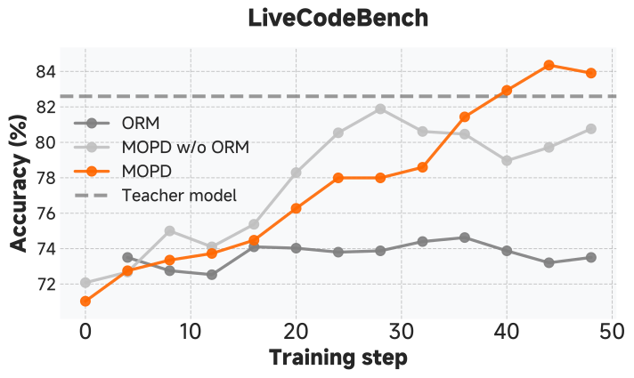
Teams can also train several domain experts, then transfer their capabilities into the main model through multi-teacher on-policy distillation (MOPD).

Training a smaller model with a stronger teacher

Qwen3 uses its 32B and 235B-A22B models as teachers for six smaller models. Those students first train on teacher-written responses, then generate their own responses for on-policy distillation. The first phase supplies reasoning and mode-switching examples; the second lets the teacher supervise how each student actually uses those abilities.

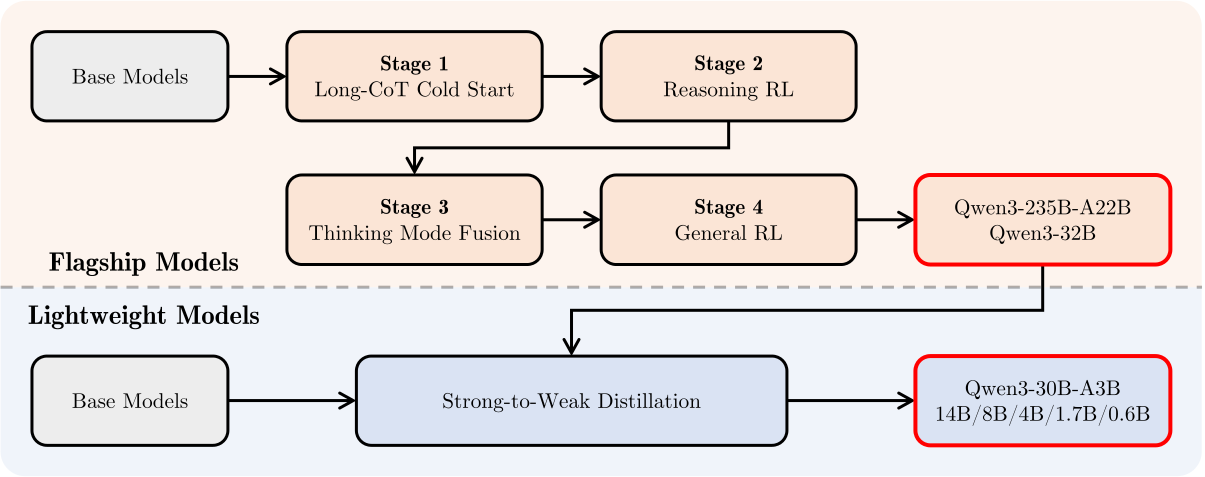
Qwen3 training pipeline: four post-training stages for the flagship models, with strong-to-weak distillation into the smaller models. — Qwen Team, Figure 1 · Original figure. The lower route shows how the smaller models learn from the flagship models.Open the image for a closer look.

Qwen3 compared reinforcement learning and on-policy distillation starting from the same off-policy distilled 8B checkpoint, with training focused on math and code. Reinforcement learning took 17,920 GPU hours to reach 67.6 on AIME’24; on-policy distillation reached 74.4 in 1,800 GPU hours. These costs cover this additional student training stage, with a trained teacher already available. [Qwen3, Table 21]

Combining specialists into one model

DeepSeek-V4 uses OPD to build the final generalist. It first trains domain specialists with supervised fine-tuning and RL, then distills more than ten teachers into one student. The student generates the trajectories; relevant experts supply supervision for domains such as mathematics and programming.

This replaces the mixed RL stage used in the previous pipeline. The report describes a weighted sum of reverse-KL losses over the full vocabulary, consolidating capabilities through output distributions instead of merging expert weights. It reports avoiding the degradation encountered with weight merging or mixed RL. RL still trains the specialists. OPD changes how their separately developed capabilities reach the model that users interact with. [DeepSeek-V4, §5.1]

Recovering abilities from earlier checkpoints

The teachers can also come from a single model’s training history. GLM-5 reports that successive RL stages can degrade previously acquired skills. It finishes with cross-stage OPD: checkpoints saved at the ends of earlier stages become teachers, and prompts are drawn from their corresponding RL training sets.

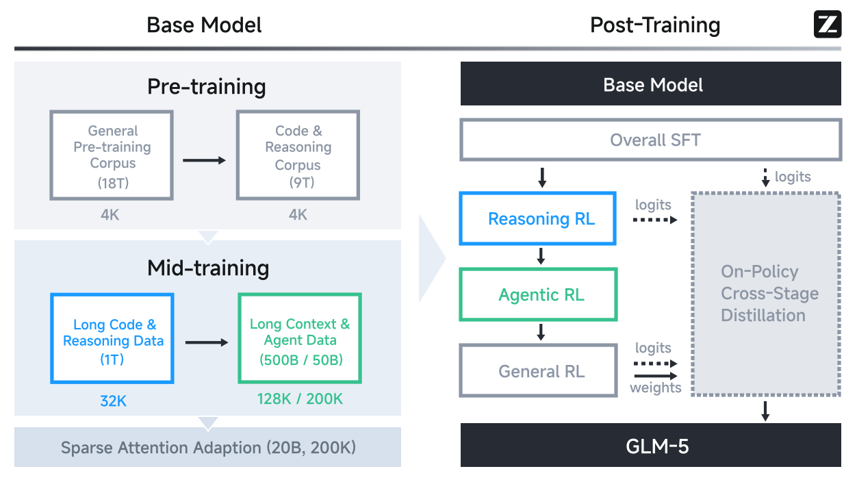
GLM-5 training pipeline, from pre-training and mid-training through SFT, successive RL stages, and on-policy cross-stage distillation. — GLM-5 Team, Figure 5 · Original figure. Follow the post-training stages to see where cross-stage distillation enters.Open the image for a closer look.

On those prompts, the current student generates responses and receives the detached teacher–student log-probability difference as its advantage. [GLM-5, §3.5]

Using teacher feedback alongside task rewards

MiMo-V2-Flash also trains domain specialists and distills them into a generalist, but its default recipe retains outcome rewards during distillation. Its pipeline makes the two sources of supervision visible:

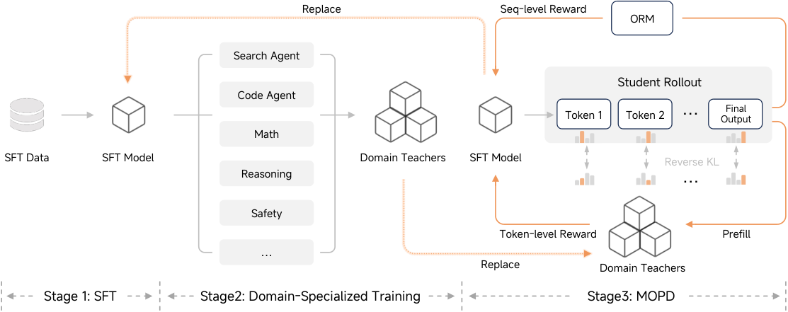
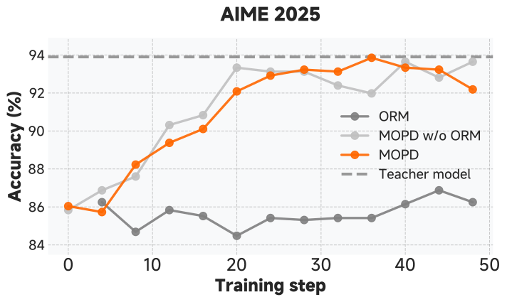
MiMo's three-stage pipeline: SFT, domain-specialized teacher training, and MOPD. The student receives sequence-level rewards from an ORM and token-level rewards from domain teachers. — MiMo Team, Figure 3 · Original figure. In Stage 3, the outcome reward model (ORM) scores the response while domain teachers supply token-level feedback.Open the image for a closer look.

The student’s update combines the token-level MOPD advantage with an outcome advantage, allowing task feedback to shape the policy during distillation. [MiMo-V2-Flash, Eq. 9 and Fig. 6]

AIME 2025 training curves comparing RL, MOPD without an outcome reward model, and MOPD. — MiMo Team, Figure 6 · Original figure. The authors compare RL, MOPD without outcome rewards, and MOPD with outcome rewards. The horizontal axis measures training steps.Open the image for a closer look.

LiveCodeBench training curves comparing RL, MOPD without an outcome reward model, and MOPD. — MiMo Team, Figure 6 · Original figure. The authors compare RL, MOPD without outcome rewards, and MOPD with outcome rewards. The horizontal axis measures training steps.Open the image for a closer look.

Open questions

The training pipelines above use OPD to reuse capabilities acquired elsewhere: in a larger model, a specialist, or an earlier checkpoint. This raises a question that the loss function alone cannot answer: what determines how much of a teacher’s ability a student can acquire, and how much computation that transfer requires? Thinking Machines offers one interpretation of OPD’s efficiency: discovering an effective strategy through RL can be much more expensive than learning it once a teacher has found it. Understanding when this shortcut works would help explain where post-training compute actually goes. [Lu et al., 2025]

A lower distillation loss tells us that the student’s predictions are closer to the teacher’s on the states being measured. It does not, by itself, explain why the student becomes better at unfamiliar problems. Earlier work on knowledge distillation found that closer agreement and better generalization do not always move together, and that optimization can prevent a student from matching a teacher even when its capacity is sufficient. For OPD, this leaves a question about what the updates accomplish: which corrections teach a reusable way of solving problems, and which mainly change how often the student produces behaviors it could already generate? [Stanton et al., 2021]

The pace of learning is also unresolved. Recent experiments found that a small set of prompts could support much of the improvement obtained with a full dataset, yet absorbing the available supervision still required hundreds of updates. Even holding the training trajectories fixed did not make alignment happen quickly. These results, currently limited to the studied models and tasks, suggest that supplying more examples need not remove the bottleneck. They leave open why useful teacher–student differences become progressively harder to absorb, and how to distinguish an optimization limit from a limit in what the student can represent. [Fu et al., 2026, §5]

There is a further choice about what to transfer. A teacher’s final policy contains both its acquired skills and its limitations. Direct-OPD explores transferring the change induced by the teacher’s RL training, using its before-and-after checkpoints, and reports improvements even when the student already outperforms the teacher. How far such transfer extends remains open. Together, these questions bear on a practical decision throughout frontier training: when should we spend more compute learning from an existing model, and when does progress require new experience and feedback from the task itself? [Feng et al., 2026]

Citation

Cited as:

Liu, Benjamin. "On-Policy Distillation". junkuanliu.com (Sep 2026).

Or:

@article{liu2026opd,
  title   = {On-Policy Distillation},
  author  = {Liu, Benjamin},
  journal = {junkuanliu.com},
  year    = {2026},
  month   = {Sep},
  url     = {https://junkuanliu.com/notes/on-policy-distillation}
}

References

[1]Pomerleau, D. (1989). ALVINN: An autonomous land vehicle in a neural network. NIPS
[2]Bagnell, J. A. (2015). An invitation to imitation. CMU Robotics Institute technical report
[3]Pomerleau, D. (1991). Efficient training of artificial neural networks for autonomous navigation. Neural Computation 3(1)
[4]Daumé III, H., Langford, J. & Marcu, D. (2009). Search-based structured prediction (SEARN). Machine Learning
[5]Osa, T. et al. (2018). An algorithmic perspective on imitation learning. Foundations and Trends in Robotics
[6]Ross, S. & Bagnell, D. (2010). Efficient reductions for imitation learning. AISTATS
[7]Ross, S., Gordon, G. & Bagnell, D. (2011). A reduction of imitation learning and structured prediction to no-regret online learning (DAgger). AISTATS
[8]Zare, M. et al. (2024). A survey of imitation learning: Algorithms, recent developments, and challenges. IEEE Transactions on Cybernetics
[9]Laskey, M. et al. (2017). DART: Noise injection for robust imitation learning. CoRL
[10]Ross, S. & Bagnell, D. (2014). Reinforcement and imitation learning via interactive no-regret learning (AggreVaTe)
[11]Buciluă, C., Caruana, R. & Niculescu-Mizil, A. (2006). Model compression. KDD
[12]Gou, J., Yu, B., Maybank, S. J. & Tao, D. (2021). Knowledge distillation: A survey. IJCV
[13]Ba, L. J. & Caruana, R. (2014). Do deep nets really need to be deep?. NeurIPS
[14]Hinton, G., Vinyals, O. & Dean, J. (2015). Distilling the knowledge in a neural network
[15]Bengio, S., Vinyals, O., Jaitly, N. & Shazeer, N. (2015). Scheduled sampling for sequence prediction with recurrent neural networks. NeurIPS
[16]Ranzato, M., Chopra, S., Auli, M. & Zaremba, W. (2016). Sequence level training with recurrent neural networks. ICLR
[17]Zhang, B. (2026). A formula-driven survey and research agenda for on-policy distillation
[18]Furlanello, T. et al. (2018). Born again neural networks. ICML
[19]Stanton, S. et al. (2021). Does knowledge distillation really work?. NeurIPS
[20]Kim, Y. & Rush, A. (2016). Sequence-level knowledge distillation. EMNLP
[21]Song, M. & Zheng, M. (2026). A survey of on-policy distillation for large language models
[22]Lin, A., Wohlwend, J., Chen, H. & Lei, T. (2020). Autoregressive knowledge distillation through imitation learning (ImitKD). EMNLP
[23]Beyer, L. et al. (2021). Knowledge distillation: A good teacher is patient and consistent. CVPR 2022
[24]Xu, X. et al. (2024). A survey on knowledge distillation of large language models
[25]Gudibande, A. et al. (2023). The false promise of imitating proprietary LLMs
[26]Agarwal, R. et al. (2023). On-policy distillation of language models: Learning from self-generated mistakes (GKD). ICLR 2024
[27]Gu, Y. et al. (2023). MiniLLM: Knowledge distillation of large language models. ICLR 2024
[28]Lu, K. & Thinking Machines Lab (2025). On-policy distillation. Connectionism
[29]Helwig, J. (2026). On-policy distillation (OPD). verl documentation
[30]DeepSeek-AI (2026). DeepSeek-V4: Towards highly efficient million-token context intelligence
[31]Zeng, A. et al. (2026). GLM-5: From vibe coding to agentic engineering
[32]Yang, A. et al. (2025). Qwen3 technical report
[33]Xiao, B. et al. (2026). MiMo-V2-Flash technical report
[34]Fu, Z. et al. (2026). Rethinking on-policy distillation of large language models II: One training example. arXiv preprint
[35]Feng, S. et al. (2026). Weak-to-strong generalization via direct on-policy distillation. arXiv preprint

On-Policy Distillation

History

How on-policy distillation works

01Probabilities → log-ratio

02Log-ratios → loss

03Loss → logit gradients

04Logit gradients → weights

On-policy distillation in frontier model training

Training a smaller model with a stronger teacher

Combining specialists into one model

Recovering abilities from earlier checkpoints

Using teacher feedback alongside task rewards

Open questions

Citation

References

Probabilities → log-ratio

Log-ratios → loss

Loss → logit gradients

Logit gradients → weights